What is Excel Traffic Light?
The global standard for a traffic light is that red means stop, and green means go. Due to this, the inherent conditioning is that red is bad, green is good, and orange is somewhere in between. Red usually denotes that there is a problem in the information which is presented, green that it is on track, and orange that it is at risk. These colors are used in many reports, Excel allows these colors to be used in its reports, in order to help the viewers focus on the problematic (red) areas. We can do these excel traffic light using Conditional Formatting in excel, which allows the user to customize the parameters for the colors.
Download all our templates |
| Excel Traffic Light using Conditional Formatting |
How to Create Excel Traffic Light?
In order to use the traffic lights in an Excel table, the following steps are required –
Step 1 : Insert Values into Excel Table
Insert the numbers into the Excel table, along with all the other relevant information. For example: the number of truck sales in 2016 by the sales people of a car dealership. Column A includes the names of the sales people, and column B the numbers of trucks they sold in 2016 –
 |
| Excel Table for Traffic lights in Excel |
Step 2 : Conditional Formatting in Excel
Choose the numbers in column B (without the header), and click on “Home -> Conditional Formatting -> Icon Sets” and then choose the traffic lights icons –
 |
| Conditional Formatting Excel for Traffic Light |
Step 3 : Traffic Lights in Excel
Once this is completed, the default traffic lights will appear next to the numbers in column B. The default parameters for the traffic lights are –
- The top 33% of the numbers (67% and up) have the Green traffic light next to them.
- The middle 34% of the numbers (less than 67% but more than 33) have the Yellow light next to them.
- The bottom 33% of the numbers have the Red light next to them.
 |
| Default Excel Traffic Light |
Customizing the Traffic Lights in Excel
Choose all the numbers in column B (without the header), and click on “Home -> Conditional Formatting -> Manage Rules”. The following menu will appear –
 |
| Conditional Formatting Excel Traffic Light |
Setting Up the Rules for Conditional Formatting
Click on the “Icon Set” so that it is colored in blue as in the picture above, and then click on the “Edit Rule” button. The following menu will appear –
 |
| Conditional Formatting Excel Rules |
In the top half of the menu (“Select a Rule Type”) leave the default as is (“Format all cells based on their values”). In the bottom half of the menu the following customization can be made –
- The “Format Style” mustn’t change from the default “Icon Sets”, otherwise the traffic lights will disappear.
- Clicking on the “Reverse Icon Order” button will cause the red light to appear at the top row, and the green one at the bottom. If the rest of the parameters stay the same, then the top third numbers will be red, and the bottom third green (no change to the yellow numbers).
- The “Icon Style” drop-down menu allows the user to change the appearance of the lights. There are many icons to choose from.
- Ticking the “Show Icon Only” box will cause the numbers to disappear from column B, and only the traffic lights will appear in the column.
Setting up the Parameters in Traffic Lights
Changing the parameters of the traffic lights requires in the bottom section of the menu, under “Display each icon according to these rules” –
- Each Icon can be changed by choosing one from the drop down menu
In the greater than or equal to drop down menu it is possible to choose whether either “>=” or only “>”. - In the “Value” field the parameter for which the first icon will appear can be chosen.
- In the “Type” drop down menu there are 4 possible parameters to choose from –
Number:
An absolute number.
Percent:
The top X% of all of the numbers in the column.
Formula:
This requires writing a formula, and the numbers which meet the requirements of the formula will have a traffic light next to them.
Percentile:
Only the numbers which will be included in the percentile chosen will have a traffic light next to them. - For example: if the first icon is a green traffic light (the default) and the following parameters are chosen: “>=”, the value field is “200” and the type is “Number” then all of the numbers in column B which are 200 or above will have the green traffic light next to them.
 |
| Parameters in Excel Traffic Light |
Best Practices for Creating Excel Traffic Light
 |
| Best Practice to Create Excel Traffic Light |
- If only one table appears in the spreadsheet, and the parameters apply to all of it, it is recommended to choose “This Worksheet” in the drop-down menu (after clicking on “Home -> Conditional Formatting -> Manage Rules”. This will ensure that all of the values in the table will adhere to the same parameters.
- Try and limit the number of icon sets to one per spreadsheet.
- The lights are dynamic, so changing the numbers in the column may cause the traffic light to change automatically.


No comments:
Post a Comment